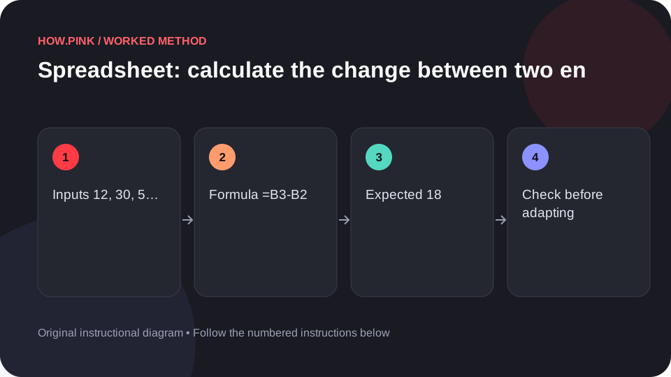
Subtract the first value from the second and retain the sign. Follow a five-row desk accessories example with the exact formula and an expected result. This worked guide uses a small reproducible example so you can check the result before adapting it to your own task.
Voordat je begint
- A spreadsheet application supporting the listed functions, such as current Excel or Google Sheets
- A blank worksheet
- Five sample rows; no private information is needed
Stapsgewijze handleiding
Create a small sample table
Open a blank worksheet. Enter these labels in column A and numbers in column B. Keep the header in row 1 and the five observations in rows 2–6.
A1: Item | B1: Quantity
A2: Pens | B2: 12
A3: Clips | B3: 30
A4: Notebooks | B4: 5
A5: Markers | B5: 8
A6: Folders | B6: 10
Keep the inputs numeric
Select B2:B6 and use a plain Number format. Enter only the number in each cell; put the unit, quantity, in the header. A value such as "12 quantity" is text and can change what numeric formulas include.
Enter the formula in a separate cell
Click D2 and type this formula, including the initial equals sign. Press Enter. Subtract the first value from the second and retain the sign. Use ordinary straight quotation marks in formulas; typographic quotation marks are not valid formula delimiters.
=B3-B2Check the worked result
With the sample data exactly as shown, D2 should return 18. If the result differs, compare the cell references and make sure the formula covers rows 2–6. Decimal results may be displayed with fewer decimal places depending on the cell format.
Adapt the range and verify a real row
Replace the sample with your own desk accessories only after the worked result matches. Expand B2:B6 and A2:A6 together when adding rows. Check one observation and one final result manually before using the worksheet.
Tips en probleemoplossing
- These examples use comma argument separators. Some regional settings require semicolons instead.
- Use straight quotes, and preserve absolute references marked with $.
- Percentage formulas return fractions; apply a Percentage format when that display is appropriate.
Veelgestelde vragen
Why does the spreadsheet show the formula instead of a result?
Change the cell format from Text to General, edit the formula, and press Enter again. Make sure the first character is =.
Can I use more than five rows?
Yes. Extend every related range to the same final row and test the result against a small subset first.